Chapter 4

Reproducing Chapter 4 of Bayesian Methods for Hackers in R + Stan

4.3 The Disorder of Small Numbers

4.3.3 Example: How to Sort Reddit Comments

The original post:

knitr::include_graphics("https://i.imgur.com/OYsHKlH.jpg")

library(tidyverse)
library(RedditExtractoR)
library(tidybayes)

reddit_thread <- reddit_content(
  "https://www.reddit.com/r/pics/comments/1w454i/deleted_by_user/"
  ) %>% 
  as_tibble()

vote_data <- reddit_thread %>% 
  mutate(
    ups = round((upvote_prop * comment_score)/(2 * upvote_prop - 1)),
    upvotes = if_else(upvote_prop != 0.5, ups, round(comment_score / 2)),
    downvotes = upvotes - comment_score,
    total_votes = upvotes + downvotes
  ) %>% 
  select(comment, comment_score, upvotes, downvotes, total_votes) %>% 
  arrange(desc(comment_score)) %>% 
  filter(comment_score > 1)

dat_lists <- vote_data %>% 
  group_by(comment) %>% 
  nest() %>% 
  mutate(data_list = map(data, compose_data))

mod <- cmdstanr::cmdstan_model("models/ch4-mod.stan")
mod$print()

data {
  int<lower=0> n;
  int upvotes[n];
  int total_votes[n];
}

parameters {
  real<lower=0,upper=1> upvote_ratio;
}

model {
  upvote_ratio ~ uniform(0, 1);
  upvotes ~ binomial(total_votes, upvote_ratio);
}

fits <- dat_lists %>% 
  mutate(
    fit = map(
      data_list, 
      ~ mod$sample(
        data = .x,
        seed = 123,
        chains = 2,
        parallel_chains = 2,
        refresh = 0
        )
      )
    )

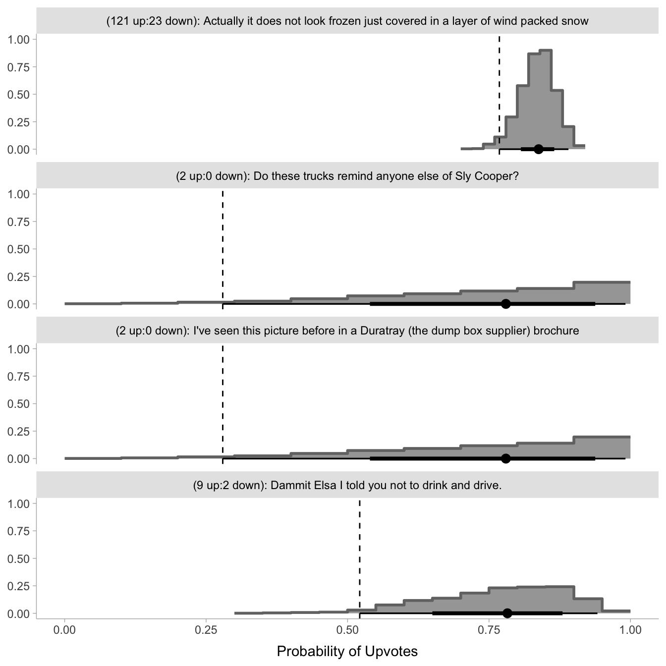
Now for visualizing some of these:

top_dists <- fits %>% 
  unnest(data) %>% 
  filter(
    str_detect(comment, "Sly Cooper") ||
      str_detect(comment, "Dammit Elsa") ||
      str_detect(comment, "Duratray") ||
      str_detect(comment, "Actually it does")
  ) %>% 
  mutate(
    draws = map(fit, ~ posterior::as_draws_df(.x$draws())),
    brief = str_sub(comment, start = 1, end = 76),
    description = paste0("(", upvotes, " up:", downvotes, " down): ", brief)
    ) %>% 
  select(description, draws) %>% 
  unnest()

Now for the histograms:

theme_set(theme_tidybayes())

least_plaus <- top_dists %>% 
  group_by(description) %>% 
  median_qi(upvote_ratio, .width = 0.95) %>% 
  select(description, .lower)
  
top_dists %>% 
  ggplot(aes(x = upvote_ratio)) +
  stat_histinterval(slab_color = "gray45") +
  facet_wrap(~ description, ncol = 1) +
  geom_vline(data = least_plaus, aes(xintercept = .lower), linetype = "dashed") +
  labs(
    y = NULL,
    x = "Probability of Upvotes"
  )

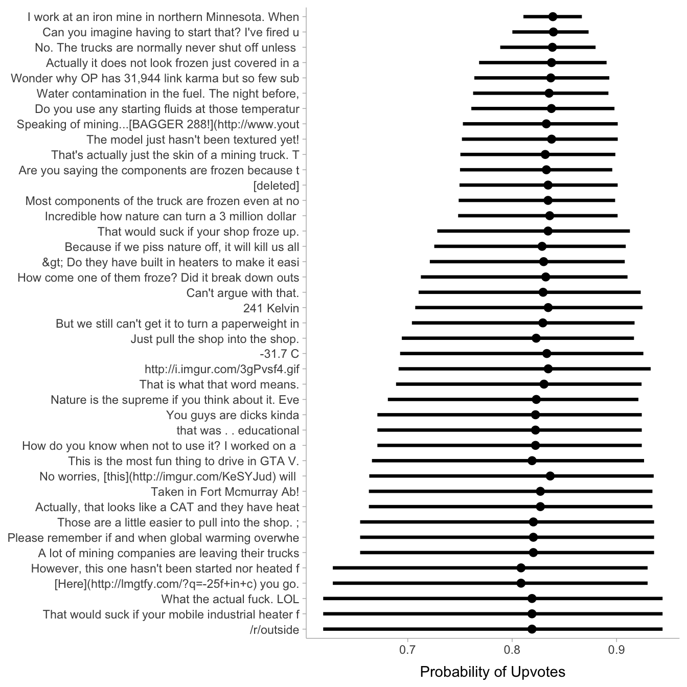
Sorting all distributions by 95% least plausible values:

all_dists <- fits %>% 
  mutate(
    draws = map(fit, ~ posterior::as_draws_df(.x$draws())),
    brief = str_sub(comment, start = 1, end = 50),
    brief = str_remove_all(brief, "\n") # remove new lines
    ) %>% 
  select(brief, draws) %>% 
  unnest(draws) %>% 
  group_by(brief) %>% 
  median_qi(upvote_ratio, .width = c(0.95)) %>% 
  mutate(
    brief = as_factor(brief),
    brief = fct_reorder(brief, .lower)
  ) %>% 
  top_n(40, .lower)

all_dists %>% 
  ggplot(aes(x = upvote_ratio, y = brief)) +
  geom_pointinterval(aes(xmin = .lower, xmax = .upper)) +
  labs(
    y = NULL,
    x = "Probability of Upvotes"
  )