3.1 The Bayesian Landscape
3.1.4 Example: Unsupervised Clustering Using a Mixture Model
library(tidyverse)
library(cmdstanr)
library(posterior)
library(bayesplot)
library(tidybayes)
library(rstan)
library(patchwork)
library(distributional)

url <- "https://raw.githubusercontent.com/CamDavidsonPilon/Probabilistic-Programming-and-Bayesian-Methods-for-Hackers/master/Chapter3_MCMC/data/mixture_data.csv"

data <- read_csv(url, col_names = FALSE) %>%
  rename(x = X1)
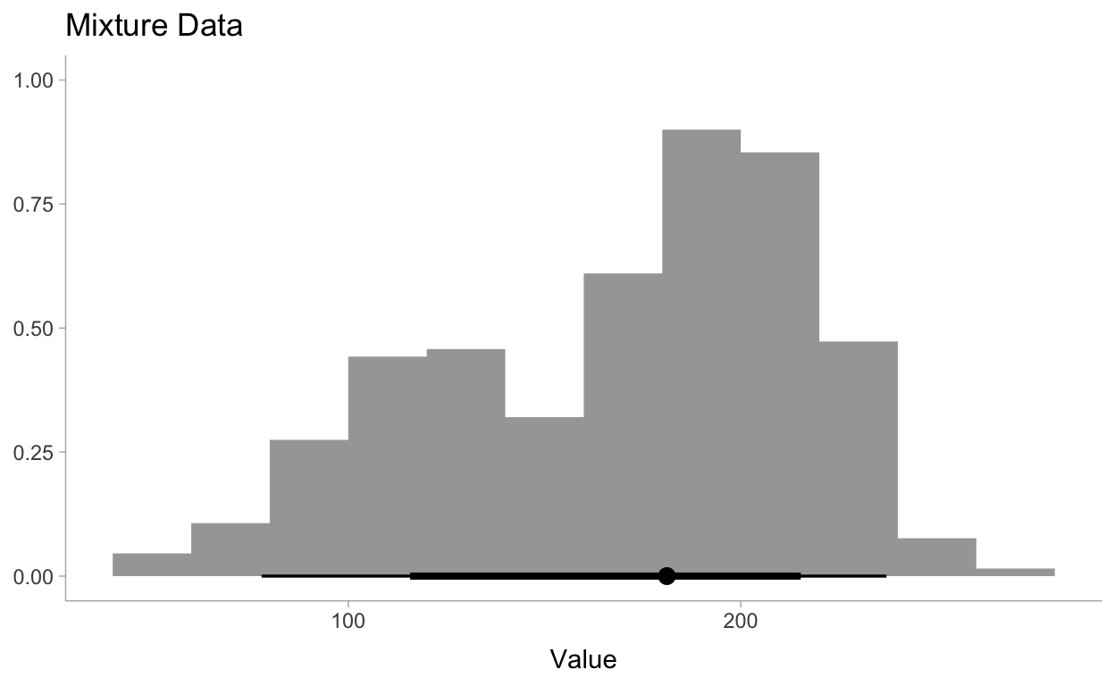
Let’s visualize this data to make sure all is well:
theme_set(theme_tidybayes())

data %>%
  ggplot(aes(x=x)) +
  stat_histinterval() +
  labs(
    title = "Mixture Data",
    x = "Value",
    y = NULL
  )
data_list <- list(
  N = 300,
  K = 2, # number of clusters
  y = data$x
)
https://mc-stan.org/docs/2_25/stan-users-guide/summing-out-the-responsibility-parameter.html
mod <- cmdstanr::cmdstan_model("models/ch3-mod.stan")
mod$print()
data {
  int<lower=1> K;          // number of mixture components
  int<lower=1> N;          // number of data points
  real y[N];               // observations
}

parameters {
  simplex[K] theta;          // mixing proportions
  ordered[K] mu;             // locations of mixture components
  vector<lower=0>[K] sigma;  // scales of mixture components
}

model {
  vector[K] log_theta = log(theta);  // cache log calculation
  sigma ~ uniform(0, 100);
  mu[1] ~ normal(120, 10);
  mu[2] ~ normal(190, 10);

  for (n in 1:N) {
    vector[K] lps = log_theta;
    for (k in 1:K)
      lps[k] += normal_lpdf(y[n] | mu[k], sigma[k]);
    target += log_sum_exp(lps);
  }
}

generated quantities {
  vector[N] yrep;
  for (i in 1:N){
    vector[K] log_theta = log(theta);
    yrep[i] = (normal_lpdf(y[i] | mu[1], sigma[1]) + log_theta[1]) >
    (normal_lpdf(y[i] | mu[2], sigma[2]) + log_theta[2]);
  }
}
fit <- mod$sample(
data = data_list,
seed = 123,
chains = 2,
parallel_chains = 2,
refresh = 1000,
iter_warmup = 4000,
iter_sampling = 8000
)
Running MCMC with 2 parallel chains...

Chain 1 Iteration:     1 / 12000 [  0%]  (Warmup)
Chain 2 Iteration:     1 / 12000 [  0%]  (Warmup)
Chain 2 Iteration:  1000 / 12000 [  8%]  (Warmup)
Chain 1 Iteration:  1000 / 12000 [  8%]  (Warmup)
Chain 1 Iteration:  2000 / 12000 [ 16%]  (Warmup)
Chain 2 Iteration:  2000 / 12000 [ 16%]  (Warmup)
Chain 1 Iteration:  3000 / 12000 [ 25%]  (Warmup)
Chain 1 Iteration:  4000 / 12000 [ 33%]  (Warmup)
Chain 1 Iteration:  4001 / 12000 [ 33%]  (Sampling)
Chain 1 Iteration:  5000 / 12000 [ 41%]  (Sampling)
Chain 1 Iteration:  6000 / 12000 [ 50%]  (Sampling)
Chain 1 Iteration:  7000 / 12000 [ 58%]  (Sampling)
Chain 1 Iteration:  8000 / 12000 [ 66%]  (Sampling)
Chain 1 Iteration:  9000 / 12000 [ 75%]  (Sampling)
Chain 1 Iteration: 10000 / 12000 [ 83%]  (Sampling)
Chain 1 Iteration: 11000 / 12000 [ 91%]  (Sampling)
Chain 1 Iteration: 12000 / 12000 [100%]  (Sampling)
Chain 1 finished in 34.0 seconds.
Chain 2 Iteration:  3000 / 12000 [ 25%]  (Warmup)
Chain 2 Iteration:  4000 / 12000 [ 33%]  (Warmup)
Chain 2 Iteration:  4001 / 12000 [ 33%]  (Sampling)
Chain 2 Iteration:  5000 / 12000 [ 41%]  (Sampling)
Chain 2 Iteration:  6000 / 12000 [ 50%]  (Sampling)
Chain 2 Iteration:  7000 / 12000 [ 58%]  (Sampling)
Chain 2 Iteration:  8000 / 12000 [ 66%]  (Sampling)
Chain 2 Iteration:  9000 / 12000 [ 75%]  (Sampling)
Chain 2 Iteration: 10000 / 12000 [ 83%]  (Sampling)
Chain 2 Iteration: 11000 / 12000 [ 91%]  (Sampling)
Chain 2 Iteration: 12000 / 12000 [100%]  (Sampling)
Chain 2 finished in 82.3 seconds.

Both chains finished successfully.
Mean chain execution time: 58.2 seconds.
Total execution time: 82.4 seconds.fit$summary()
# A tibble: 307 x 10
   variable     mean   median     sd    mad       q5      q95  rhat
   <chr>       <dbl>    <dbl>  <dbl>  <dbl>    <dbl>    <dbl> <dbl>
 1 lp__     -1.54e+3 -1.54e+3 1.67   1.47   -1.54e+3 -1.53e+3  1.00
 2 theta[1]  3.77e-1  3.73e-1 0.0507 0.0475  3.01e-1  4.65e-1  1.00
 3 theta[2]  6.23e-1  6.27e-1 0.0507 0.0475  5.35e-1  6.99e-1  1.00
 4 mu[1]     1.20e+2  1.20e+2 5.71   5.31    1.12e+2  1.30e+2  1.00
 5 mu[2]     2.00e+2  2.00e+2 2.62   2.64    1.95e+2  2.04e+2  1.00
 6 sigma[1]  3.02e+1  2.98e+1 4.07   3.80    2.44e+1  3.77e+1  1.00
 7 sigma[2]  2.28e+1  2.28e+1 1.91   1.87    1.99e+1  2.61e+1  1.00
 8 yrep[1]   1.00e+0  1.00e+0 0      0       1.00e+0  1.00e+0 NA
 9 yrep[2]   8.40e-1  1.00e+0 0.367  0       0.       1.00e+0  1.00
10 yrep[3]   2.75e-3  0.      0.0524 0       0.       0.       1.00
# … with 297 more rows, and 2 more variables: ess_bulk <dbl>,
#   ess_tail <dbl>
posterior <- fit$output_files() %>%
read_stan_csv()
p1 <- posterior %>%
  mcmc_trace(pars = c("mu[1]", "mu[2]")) +
  labs(
    title = "Traces of center for each cluster"
  )

p2 <- posterior %>%
  mcmc_trace(pars = c("sigma[1]", "sigma[2]")) +
  labs(
    title = "Traces of standard deviation of each cluster"
  )

p3 <- posterior %>%
  mcmc_trace(pars = c("theta[1]")) +
  labs(
    title = "Frequency of assignment to cluster 1"
  )

p1 / p2 / p3
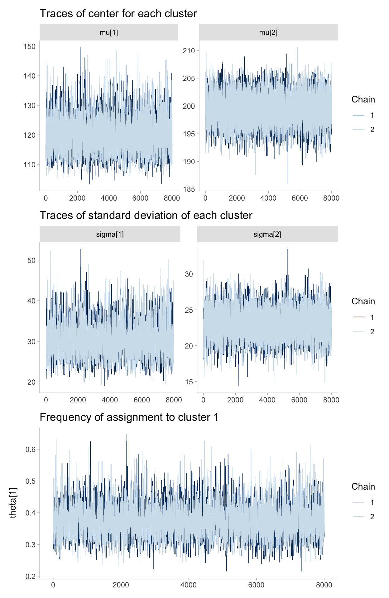
Notice the following characteristics:
- The traces converges, not to a single point, but to a distribution of possible points. This is convergence in an MCMC algorithm.
- Inference using the first few thousand points is a bad idea, as they are unrelated to the final distribution we are interested in. Thus is it a good idea to discard those samples before using the samples for inference. We call this period before converge the burn-in period.
- The traces appear as a random “walk” around the space, that is, the paths exhibit correlation with previous positions. This is both good and bad. We will always have correlation between current positions and the previous positions, but too much of it means we are not exploring the space well. This will be detailed in the Diagnostics section later in this chapter.
Cluster Investigation
# https://mpopov.com/blog/2020/09/07/pivoting-posteriors/
tidy_draws.CmdStanMCMC <- function(model, ...) {
  return(as_draws_df(model$draws()))
}
fit %>%
  gather_draws(mu[cluster], sigma[cluster]) %>%
  mutate(cluster = paste0("Cluster ", cluster)) %>%
  ggplot(aes(.value)) +
  stat_histinterval() +
  facet_wrap(vars(cluster, .variable), ncol = 2, scales = "free") +
  labs(
    title = "Posterior of center and standard deviation of clusters 1 & 2",
    y = NULL,
    x = NULL
  )
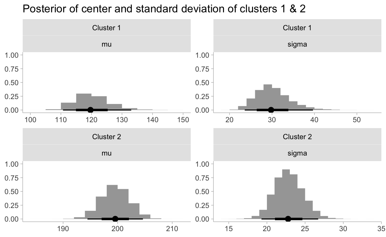
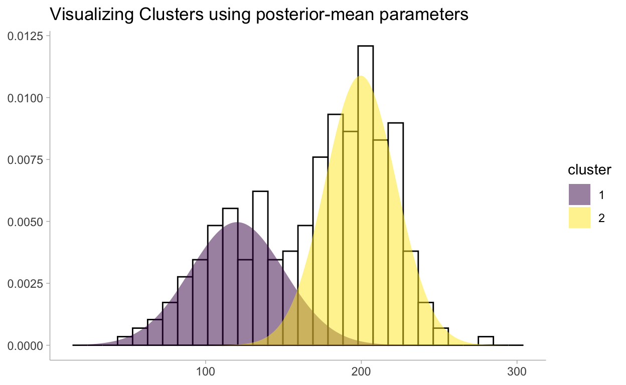
One quick and dirty way (which has nice theoretical properties we will see in Chapter 5), is to use the mean of the posterior distributions. Below we overlay the Normal density functions, using the mean of the posterior distributions as the chosen parameters, with our observed data:
distdata <- fit %>%
  spread_draws(mu[cluster], sigma[cluster], theta[cluster]) %>%
  mean_hdci() %>%
  mutate(
    cluster = as_factor(cluster),
    nest(tibble(x = seq(20, 300, length.out = 500)))
    ) %>%
  mutate(
    data = pmap(
      list(data, mu, sigma, theta),
      function(data, mu, sigma, theta)
        mutate(data, dens = theta * dnorm(x, mean = mu, sd = sigma))
      )
  ) %>%
  unnest()

distdata %>%
  ggplot(aes(x = x)) +
  geom_histogram(
    data = data,
    aes(y = stat(density)), color = "black", fill = "white"
    ) +
  geom_ribbon(aes(ymin = 0, ymax = dens, fill = cluster), alpha = 0.5) +
  labs(
    title = "Visualizing Clusters using posterior-mean parameters",
    y = NULL,
    x = NULL
  ) +
  scale_fill_viridis_d()
Returning to Clustering: Prediction
We can try a less precise, but much quicker method. We will use Bayes’ Theorem for this. As you’ll recall, Bayes’ Theorem looks like:
\[ P(A|X) = \frac{P(X|A)P(A)}{P(X)} \]
For a particular sample set of parameters for our posterior distribution, (\(\mu_1,\sigma_1,\mu_2,\sigma_2,\theta\)), we are interested in asking, “Is the probability that \(x\) is in the cluster 1 greater than the probability it is in cluster 0?” where the probability is dependent on the chosen parameters:
\[ \frac{P(x = ?|L_x = 1)P(L_x=1)}{P(x=?)} > \frac{P(x = ?|L_x = 2)P(L_x=2)}{P(x=?)} \]
Since the denominators are equal, they can be ignored:
\[
P(x = ?|L_x = 1)P(L_x=1) > P(x = ?|L_x = 2)P(L_x=2)
\] This is what you’ll see in the generated quantities block but instead on the log space. There is likely a more precise way to estimate the probability of the data points belonging to each cluster. I think it would be similar to what was done in the Chapter 1 model for the change point detection.
dataorig <- data %>%
mutate(i = row_number())
probassign <- fit %>%
gather_draws(yrep[i]) %>%
mean_hdci() %>%
left_join(dataorig)
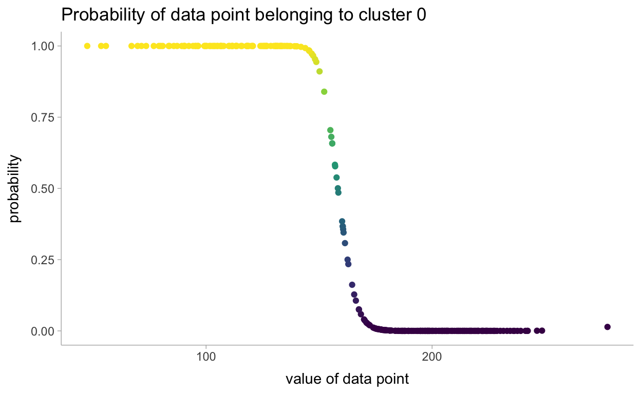
probassign %>%
ggplot(aes(x = x, y = .value)) +
geom_point(aes(color = .value)) +
scale_color_viridis_c() +
labs(
title = "Probability of data point belonging to cluster 0",
y = "probability",
x = "value of data point"
) +
theme(legend.position = "none")